How to Read a Seismogram

Převzato z https://earthquakes.berkeley.edu/blog/2012/01/01/how-to-read-a-seismogram-2.html.

January 1, 2012

During the past two weeks the Earth was seismically exceptionally quiet – until Tokyo and parts of Japan's east coast were shaken on New Year's Day. Although high rise buildings in Japanese cities swayed in a gentle fashion, no damage was reported and no tsunami was generated. The cause was an earthquake under the Western Pacific, about 300 miles southwest of Tokyo. The focus of the quake with a magnitude of 6.8 lay in the Earth's upper mantle, almost 220 miles below the ocean surface. Such deep temblors rarely cause damage because most of the waves' energy is absorbed and dissipates before the shaking reaches the Earth's surface.

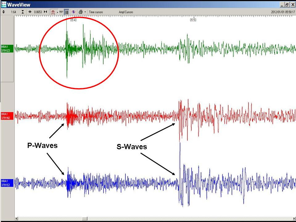
Nearly 12 minutes after the quake started, the first seismic waves hit California. The recordings of these waves with the broadband seismometers of the Berkeley Digital Seismic Network allows the blogger to make good on a promise he made a while ago, namely to further explore how to read a seismogram. Figure 22.6 shows a half hour long record of the seismic waves registered by a three component seismic station in the East Bay Hills. Green is the vertical ground movement, up and down. The red line represents the seismic shaking in the North-South and the blue line in the East-West direction. The most prominent onsets are the P- and S-waves, which arrived approximately 9.5 minutes apart. However, looking at the vertical component one can clearly see more onsets (red circle).

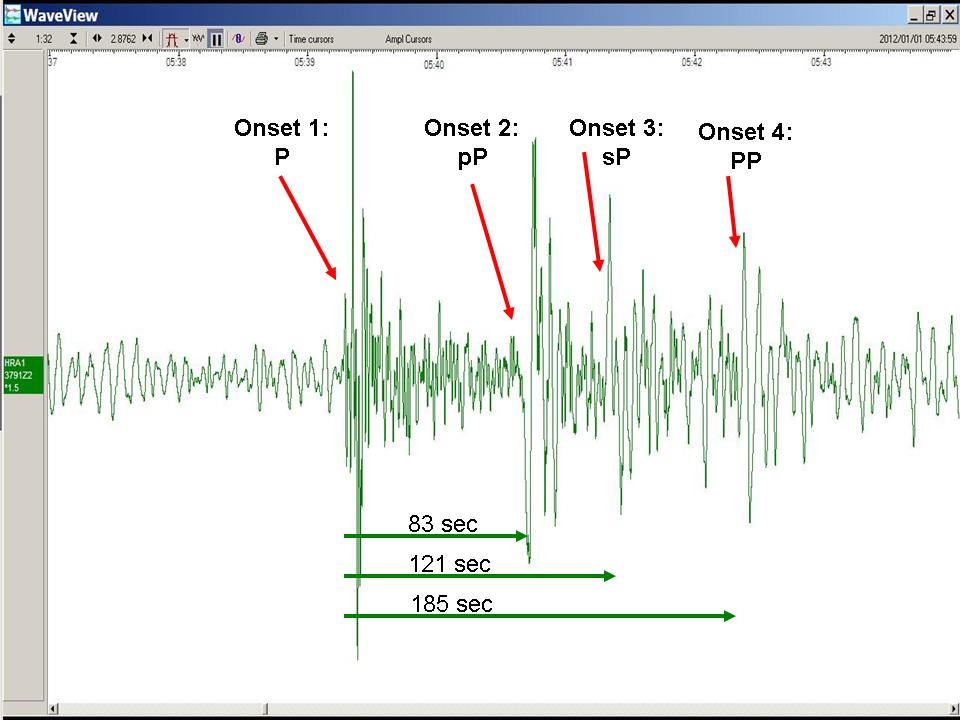
When zooming into this area of the seismogram (figure 22.7, seven minute window) four prominent peaks stand out. Each of them is called an onset, because it represents the arrival of a distinct type of seismic wave. Over the last decades, seismologists have learned how to distinguish between these various types and how to interpret their differences.

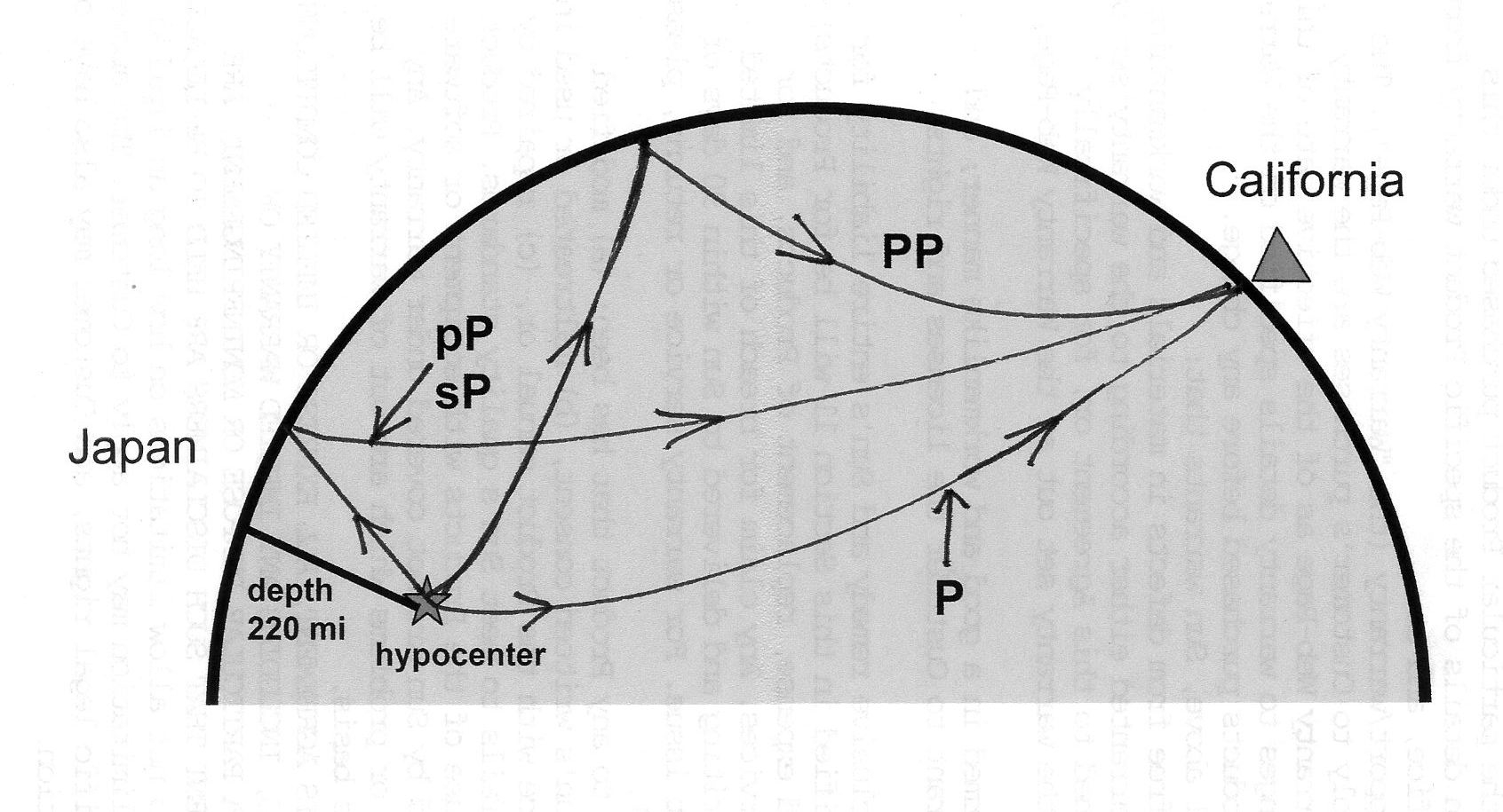
Take onsets 1 and 2 for instance: Onset 1 is the most direct wave between the quake's hypocenter and California, commonly labeled as “P” for primary. Eighty-three seconds later, another wave arrives. This wave travelled from the quake's focus initially to the surface of the Earth immediately above the hypocenter. There it was reflected and then followed the original P-wave on its way to California. This type of wave is referred to as “little p – big P” (pP). The sketch in figure 22.8 shows its idealized path.

Onset 3 is generated by a wave which first travelled as a S-wave to the Earth's surface above the focus. There, upon reflection, it was converted into a P-wave, which followed its two predecessors across the Pacific. Because of the conversion from S to P, this onset is labeled “little s – big P” (sP). Finally, the fourth onset is generated by a wave, which was reflected from the Earth's surface roughly halfway between the hypocenter and California. This wave is referred to as PP and takes more than 100 seconds longer to cross the Pacific than the immediate P-wave.

Questions:

1. Compare the speed of propagation of all these types of waves.
2. Explain why the P-wave causes vibrations in all three directions in California.
3. Assuming that the speed of propagation of the P-wave is constant, use the information in the article to calculate the speed of these waves.
4. Calculate the speed of propagation of S-waves.